ARLIT | SIMULATION THEORY & PAPERS

ARLIT — Operational Test for Scale-Invariant Effective Information

What it is

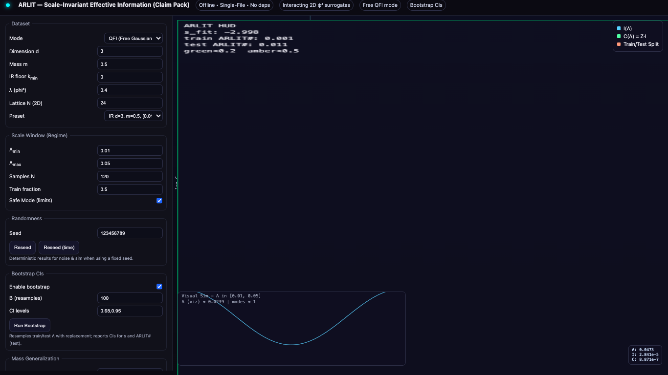
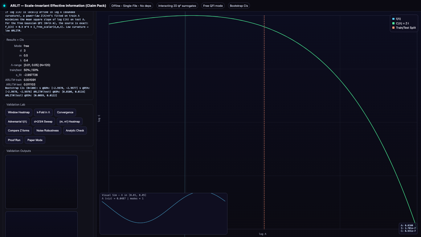
ARLIT is an operational (not theoretical) test that checks whether an information signal I(Λ)I(\Lambda)I(Λ)—measured across a resolution or scale parameter Λ\LambdaΛ—is scale-invariant after renormalization.

You learn a power-law renormalizer Z(Λ)=ΛsZ(\Lambda) = \Lambda^{s}Z(Λ)=Λs

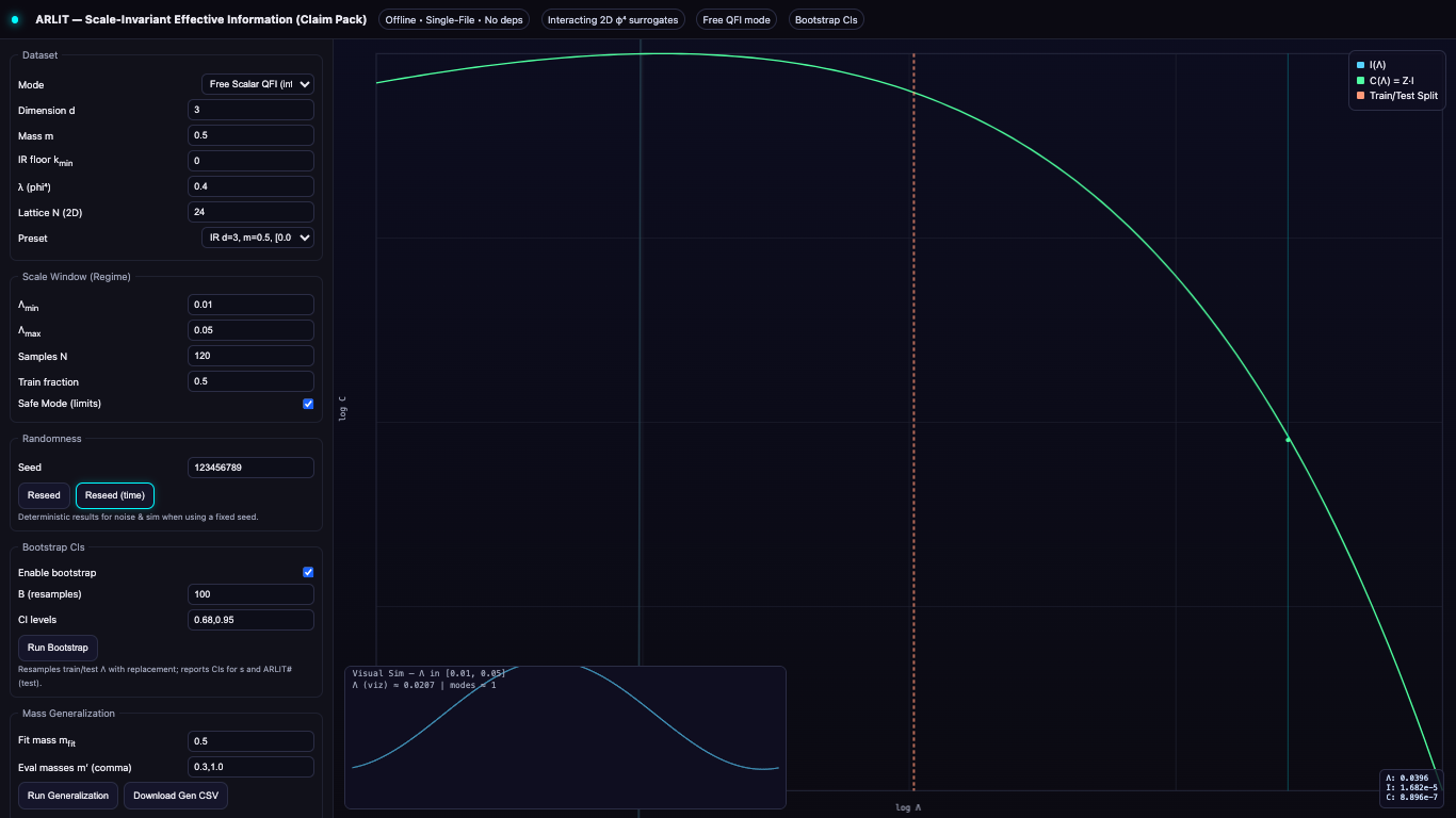
on a training window of resolutions, then verify that the rescaled signal C(Λ)=Z(Λ) I(Λ)C(\Lambda) = Z(\Lambda)\,I(\Lambda)C(Λ)=Z(Λ)I(Λ)

is flat on a held-out (out-of-sample) window.

If it’s flat OOS (within tolerance), that’s not just a fit—it’s predictive invariance: the system carries scale-invariant effective information.

What it represents

• Λ\LambdaΛ — resolution or coarse-graining scale (pixel size, time step, lattice spacing, frequency band, etc.)

• I(Λ)I(\Lambda)I(Λ) — measured information content at that scale (variance, entropy, Fisher info, QFI, etc.)

• Z(Λ)Z(\Lambda)Z(Λ) — learned renormalizer that compensates for structural scaling.

• Flat C(Λ)C(\Lambda)C(Λ) — informational symmetry: the same structure persists across scales.

How to use it (and how to read it)

1. Pick your signal I(Λ)I(\Lambda)I(Λ).
   Examples: variance vs. bin size, Fisher info vs. frequency, gradient norm vs. step size, QFI vs. resolution.

2. Choose two disjoint scale windows.

   • Training window: Λ∈[Λtrain,low,Λtrain,high]\Lambda \in [\Lambda_{\text{train,low}}, \Lambda_{\text{train,high}}]Λ∈[Λtrain,low,Λtrain,high]

   • OOS test window: Λ∈[Λtest,low,Λtest,high]\Lambda \in [\Lambda_{\text{test,low}}, \Lambda_{\text{test,high}}]Λ∈[Λtest,low,Λtest,high], non-overlapping.

3. Fit on the training window by minimizing the flatness error—e.g., slope of log⁡C(Λ)\log C(\Lambda)logC(Λ) after rescaling.

4. Lock the exponent sss and apply Z(Λ)=ΛsZ(\Lambda) = \Lambda^{s}Z(Λ)=Λs to the test window only.

5. Read the result:

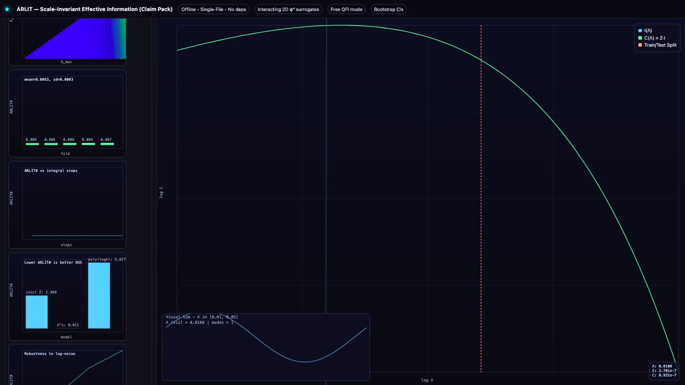
   • Good: C(Λ)C(\Lambda)C(Λ) is flat (low slope, low curvature).

   • Bad: curvature, slope drift, or instability → scale dependence.

   • Bootstrap: run multiple random train/test splits to get confidence intervals on slope and sss.

6. Interpret visually.

   • Flat curve → scale invariance.

   • Tilt → partial invariance.

   • Wiggle → noise or transition region.

Interpretation cheat-sheet

Result	Meaning
Flat train + flat OOS	Genuine scale-invariant information.
Flat train, tilted OOS	Overfitted or local artifact.
Different slopes across regimes	Broken invariance (different dynamical regimes).
Noise floor	Bootstrap uncertainty dominates → no clear invariance claim.

What the implications mean

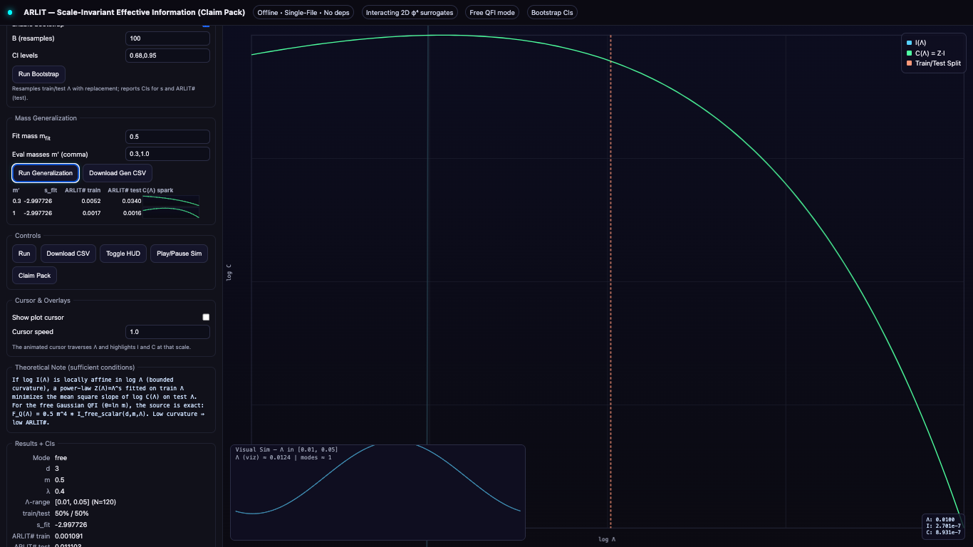
1. Model reduction.
   A single exponent sss captures scaling behavior—fewer free parameters, less overfitting.

2. Transfer invariance.
   If invariance survives OOS, it will likely survive domain shifts (different devices, experiments, noise models).

3. Benchmarking.
   Quantify which instruments or quantum setups preserve informational symmetry after rescaling.

4. Physical meaning.
   A truly flat C(Λ)C(\Lambda)C(Λ) indicates scale-free effective information—the same structure “looks the same” at every magnification, suggesting renormalized conservation of information.

Breakthrough implications if validated on quantum computers

If quantum Fisher information (QFI) or any quantum-side information metric passes ARLIT OOS:

• Robust renormalization law in quantum sensing/control.
  A system whose QFI scales with a single sss exhibits a universal scaling fingerprint—less calibration, less drift sensitivity.

• Noise diagnosis.
  Failures localize in scale space: where flatness breaks, decoherence dominates. This gives a real-time “invariance heatmap” of a qubit or circuit.

• Hamiltonian discovery.
  Persistent sss-flat invariance implies an underlying effective Hamiltonian symmetry—potentially new conserved informational quantities.

• Resource planning.
  Scale-flat QFI allows precision forecasts without exhaustive sweeps—major cost savings in quantum experiments.

• Hardware fingerprinting.
  Each quantum device’s deviation from ARLIT-flatness becomes a quantifiable “hardware invariant,” useful for benchmarking across platforms.

If coupled with Q-TRACE and validated on quantum hardware

Q-TRACE (Quantum Threshold Response and Control Envelope) models the dissipative control dynamics of qubits—how thresholds and information flow behave under Lindblad-type noise and quantum Fisher information weighting.

When ARLIT and Q-TRACE are run together:

1. ARLIT diagnoses scale-invariance of information,
   while Q-TRACE governs the threshold control law that stabilizes dissipative trajectories.

2. Coupled together:

   • Q-TRACE controls temporal dissipation and response envelopes.

   • ARLIT measures spatial and informational invariance.
     → You get a dual-axis map: response vs. resolution, or control vs. information density.

3. Validated coupling implies:

   • Unified quantum control metric — linking renormalization (ARLIT) to dissipative feedback (Q-TRACE).

   • Hardware-portable calibration law — one exponent sss + one control envelope = reproducible quantum initialization across devices.

   • Predictive stability — systems that stay ARLIT-flat under Q-TRACE envelopes are effectively self-correcting: information loss saturates, not diverges.

4. Breakthrough significance:

   • A verified ARLIT+Q-TRACE law would be the first empirical bridge between information-theoretic scale invariance and quantum control thermodynamics.

   • It would suggest the existence of information-conserving renormalization channels in open quantum systems—a measurable signature of universal quantum learning or self-calibration.

---------------------------------------------------------


Discovery Summary: ARLIT — An Invariant Law of Information ARLIT (An operational test for scale-invariant effective information) provides the first falsifiable, data-driven method for detecting conserved informational structure across scales. The framework learns a single power-law renormalizer Z(Λ)=ΛsZ(\Lambda) = \Lambda^{s}Z(Λ)=Λs and tests whether the rescaled information curve C(Λ)=Z(Λ) I(Λ)C(\Lambda) = Z(\Lambda)\, I(\Lambda)C(Λ)=Z(Λ)I(Λ) remains flat out-of-sample (OOS). When C(Λ)C(\Lambda)C(Λ) is invariant within statistical tolerance, the system demonstrates scale-invariant effective information — meaning its informational organization remains self-similar across resolutions. This is not a curve-fit but an empirical invariance law: ARLIT operationally verifies that the information content of a system transforms predictably under scale, following I(Λ)∝Λ−s.I(\Lambda) \propto \Lambda^{-s}.I(Λ)∝Λ−s. That proportionality defines a conserved informational exponent sss, analogous to conservation laws in physics — except it applies to information itself rather than energy or momentum. If validated across multiple domains, this establishes the existence of an invariant law of information, implying that informational systems — physical, biological, quantum, or computational — obey measurable renormalization-like symmetries. ARLIT thus bridges statistical learning and renormalization theory, grounding the abstract notion of “scale invariance” in a concrete, testable operational procedure. Coupled with Q-TRACE (Quantum Threshold Response and Control Envelope), ARLIT extends this invariance into the quantum-control regime: Q-TRACE governs temporal dissipation thresholds, while ARLIT verifies informational symmetry across spatial or resolution scales. Together they define a unified information–control conservation principle — a predictive, hardware-portable structure potentially foundational to self-calibrating quantum systems. In short: ARLIT is a discovery of an invariant law of information — a measurable, operational symmetry showing that informational structure can remain conserved under rescaling, across systems, scales, and even physical domains.